An introduction to Computer Vision in Python

This post is based off a talk I gave last week to the Perth Python meetup group. You can either read the quick written version of the talk below, or head to GitHub for the slides and Jupyter notebooks.

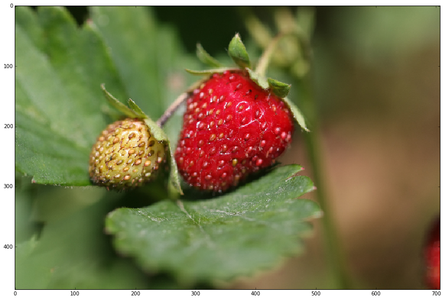
We'll walk through a simple solution to the problem faced by a robotic strawberry picking robot - locate the largest strawberry in the scene and find it's rough size, position and orientation.

Getting started

First, we need to install OpenCV. If you're on OS X you can use Homebrew with brew install opencv3 --with-python, or if you're on Windows then you can use Anaconda: conda install opencv3.

Then we can import some libraries - we're importing OpenCV (cv2), numpy and matplotlib. Since this was developed in a Jupyter notebook, I've added the %matplotlib inline magic to get my matplotlib plots to show up in the notebook.

%matplotlib inline
import cv2
import matplotlib
from matplotlib import colors
from matplotlib import pyplot as plt
import numpy as np
from __future__ import division

Basics

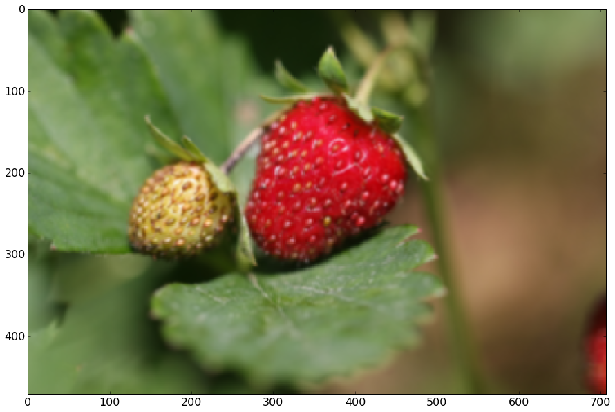
First off, let's load an image:

image = cv2.imread('strawberries.jpg')

Images in OpenCV are represented as numpy arrays - image.shape shows us that the image is 1414 pixels high, by 2121 pixels wide, and we get three channels - they're loaded in as [B, G, R].

image.shape

(1414, 2121, 3)

Let's convert it to RGB so we can display it (matplotlib's imshow expects RGB), and resize it to be a bit more of a manageable size:

# Convert from BGR to RGB
image = cv2.cvtColor(image, cv2.COLOR_BGR2RGB)

# Resize to a third of the size
image = cv2.resize(image, None, fx=1/3, fy=1/3)

Now we can show the image - we create a matplotlib figure with a maximum size of 15x15 inches, and then show the image:

def show(image):
    # Figure size in inches
    plt.figure(figsize=(15, 15))

    # Show image, with nearest neighbour interpolation
    plt.imshow(image, interpolation='nearest')

show(image)

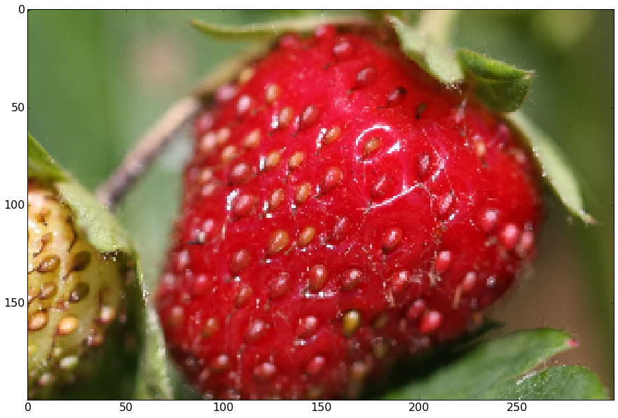
We can also crop the image with the slice syntax, the same way we'd manipulate a numpy array:

image_cropped = image[100:300, 200:500]
show(image_cropped)

Colour spaces

Since we're trying to find the red strawberry, we can look at each of the Red/Green/Blue channels individually. Here we're zeroing out the other channels:

# Show Red/Green/Blue
images = []
for i in [0, 1, 2]:
    colour = image.copy()
    if i != 0: colour[:,:,0] = 0
    if i != 1: colour[:,:,1] = 0
    if i != 2: colour[:,:,2] = 0
    images.append(colour)

show(np.vstack(images))

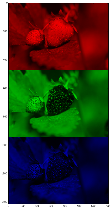
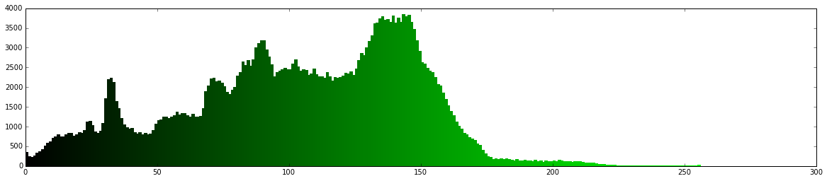
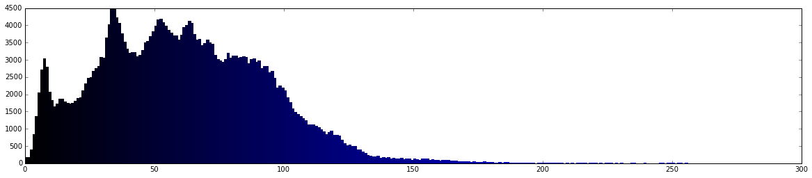
It's not super clear by looking at these that we'll be able to easily distinguish the strawberry from the background by using RGB - let's look at a histogram:

def show_rgb_hist(image):
    colours = ('r','g','b')
    for i, c in enumerate(colours):
        plt.figure(figsize=(20, 4))
        histr = cv2.calcHist([image], [i], None, [256], [0, 256])

        if c == 'r': colours = [((i/256, 0, 0)) for i in range(0, 256)]
        if c == 'g': colours = [((0, i/256, 0)) for i in range(0, 256)]
        if c == 'b': colours = [((0, 0, i/256)) for i in range(0, 256)]

        plt.bar(range(0, 256), histr, color=colours, edgecolor=colours, width=1)

        plt.show()

show_rgb_hist(image)

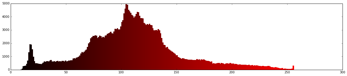
Let's try HSV - this separates Hue into the first channel, and Saturation and Value as the second two channels:

# Convert from RGB to HSV
hsv = cv2.cvtColor(image, cv2.COLOR_RGB2HSV)

images = []
for i in [0, 1, 2]:
    colour = hsv.copy()
    if i != 0: colour[:,:,0] = 0
    if i != 1: colour[:,:,1] = 255
    if i != 2: colour[:,:,2] = 255
    images.append(colour)

hsv_stack = np.vstack(images)
rgb_stack = cv2.cvtColor(hsv_stack, cv2.COLOR_HSV2RGB)
show(rgb_stack)

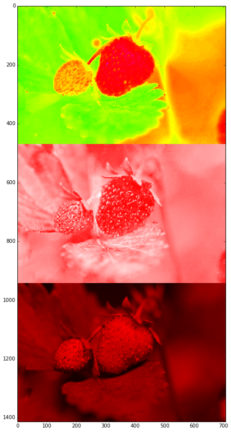
The hue image above looks quite promising - we should be able to filter by hue to extract the red bit from the green background.

matplotlib.rcParams.update({'font.size': 16})

def show_hsv_hist(image):
    # Hue
    plt.figure(figsize=(20, 3))
    histr = cv2.calcHist([image], [0], None, [180], [0, 180])
    plt.xlim([0, 180])
    colours = [colors.hsv_to_rgb((i/180, 1, 0.9)) for i in range(0, 180)]
    plt.bar(range(0, 180), histr, color=colours, edgecolor=colours, width=1)
    plt.title('Hue')

    # Saturation
    plt.figure(figsize=(20, 3))
    histr = cv2.calcHist([image], [1], None, [256], [0, 256])
    plt.xlim([0, 256])

    colours = [colors.hsv_to_rgb((0, i/256, 1)) for i in range(0, 256)]
    plt.bar(range(0, 256), histr, color=colours, edgecolor=colours, width=1)
    plt.title('Saturation')

    # Value
    plt.figure(figsize=(20, 3))
    histr = cv2.calcHist([image], [2], None, [256], [0, 256])
    plt.xlim([0, 256])

    colours = [colors.hsv_to_rgb((0, 1, i/256)) for i in range(0, 256)]
    plt.bar(range(0, 256), histr, color=colours, edgecolor=colours, width=1)
    plt.title('Value')

show_hsv_hist(hsv)

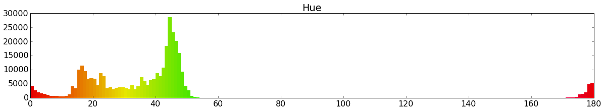
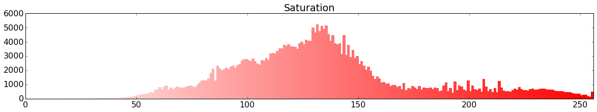
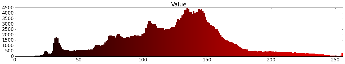
So from the histograms above we can see that we should be filtering between around 0-10 and 170-180 in Hue, and since we want to pick up the bright red strawberry we should filter saturation and value to above around 100-150.

We'll get better results if we blur slightly first:

# Blur image slightly
image_blur = cv2.GaussianBlur(image, (7, 7), 0)
show(image_blur)

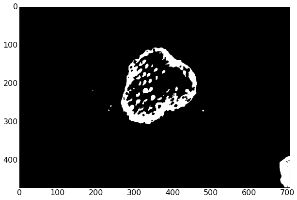
Filtering by colour

Now we can convert our RGB blurred image to HSV, and filter by the range 0-10 hue, 100-256 saturation, and 80-256 value:

image_blur_hsv = cv2.cvtColor(image_blur, cv2.COLOR_RGB2HSV)

# 0-10 hue
min_red = np.array([0, 100, 80])
max_red = np.array([10, 256, 256])
image_red1 = cv2.inRange(image_blur_hsv, min_red, max_red)

To make our lives a little easier let's define a show_mask function for showing a binary image:

def show_mask(mask):
    plt.figure(figsize=(10, 10))
    plt.imshow(mask, cmap='gray')

show_mask(image_red1)

Now let's do the same for 170-180 hue:

# 170-180 hue
min_red2 = np.array([170, 100, 80])
max_red2 = np.array([180, 256, 256])
image_red2 = cv2.inRange(image_blur_hsv, min_red2, max_red2)

show_mask(image_red2)

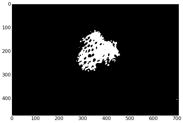
And since these are binary images (values either 0 or 255) of the same size, we can add them together:

image_red = image_red1 + image_red2
show_mask(image_red)

Cleanup

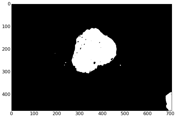
Our mask looks pretty good - we've got most of the strawberry selected, but there are some voids and some extra specks around. We can use a technique known as morphology to close (fill voids) and then open (remove small specks). Here we're using a circle of size 15 - this is big enough to remove all the specks and fill all the voids - if it was any bigger it would start to distort the shape of the strawberry.

kernel = cv2.getStructuringElement(cv2.MORPH_ELLIPSE, (15, 15))

# Fill small gaps
image_red_closed = cv2.morphologyEx(image_red, cv2.MORPH_CLOSE, kernel)
show_mask(image_red_closed)

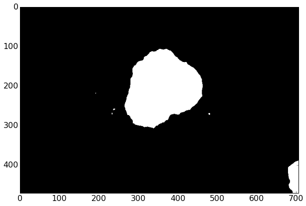
# Remove specks
image_red_closed_then_opened = cv2.morphologyEx(image_red_closed, cv2.MORPH_OPEN, kernel)
show_mask(image_red_closed_then_opened)

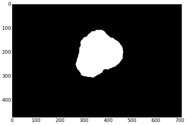
Finding the biggest contour

Since our image might have multiple strawberries in it, or some small red blobs, we can grab just the largest contour (continous shape):

def find_biggest_contour(image):

    # Copy to prevent modification
    image = image.copy()
    contours, hierarchy = cv2.findContours(image, cv2.RETR_LIST, cv2.CHAIN_APPROX_SIMPLE)

    # Isolate largest contour
    biggest_contour = max(contours, key=cv2.contourArea)

    # Draw just largest contour
    mask = np.zeros(image.shape, np.uint8)
    cv2.drawContours(mask, [biggest_contour], -1, 255, -1)
    return biggest_contour, mask

big_contour, mask = find_biggest_contour(image_red_closed_then_opened)
show_mask(mask)

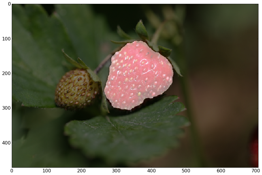
Now we can show the mask overlaid on the original image by adding the two together. We have to convert the mask to RGB because we can only add arrays of the same shape.

def overlay_mask(mask, image):
    rgb_mask = cv2.cvtColor(mask, cv2.COLOR_GRAY2RGB)
    img = cv2.addWeighted(rgb_mask, 0.5, image, 0.5, 0)
    show(img)

overlay_mask(mask, image)

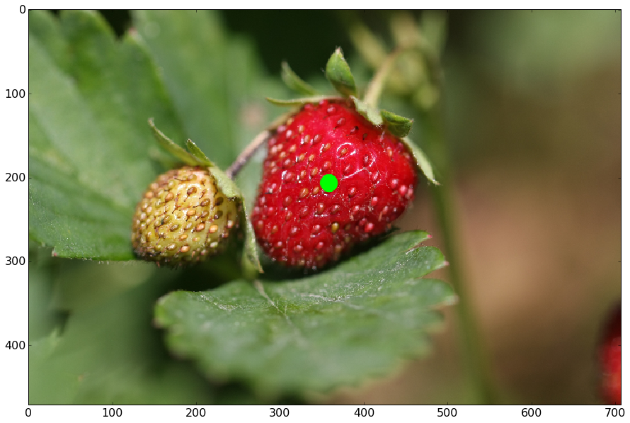
Final results

Now we can figure out where the center of mass of the strawberry is using it's moments.

# Centre of mass
moments = cv2.moments(mask)
centre_of_mass = (
    int(moments['m10'] / moments['m00']),
    int(moments['m01'] / moments['m00'])
)
image_with_com = image.copy()
cv2.circle(image_with_com, centre_of_mass, 10, (0, 255, 0), -1, cv2.CV_AA)
show(image_with_com)

And draw an ellipse around it - this is a useful way to get the size and orientation of the strawberry.

# Bounding ellipse
image_with_ellipse = image.copy()
ellipse = cv2.fitEllipse(big_contour)
cv2.ellipse(image_with_ellipse, ellipse, (0, 255, 0), 2)
show(image_with_ellipse)

My slides, all the source code (in Jupyter notebooks), and some demos from the talk are available on GitHub: https://github.com/alexlouden/strawberries

Please let me know what you think!